大家好,我是带我去滑雪!
随着精准医疗和个体化治疗的快速发展,传统的组织学分型已逐渐无法满足对脑胶质瘤这一复杂疾病的深度理解。低级别胶质瘤(Low-Grade Glioma, LGG)是一种生长缓慢但潜在恶性的脑部肿瘤,其生物学行为和临床预后高度依赖于肿瘤的分子亚型特征,如IDH基因突变、1p/19q共缺失、MGMT启动子甲基化状态以及通过RNA表达、CNV等维度定义的多组学分型。近年来,随着世界卫生组织(WHO)对脑肿瘤分类标准的不断更新,分子层面的特征逐渐成为胶质瘤诊断和治疗决策的核心依据。
与此同时,磁共振成像(MRI)作为一种无创、高分辨率的成像方式,已成为胶质瘤临床诊断、疗效评估与手术导航的关键手段。研究发现,不同分子亚型的LGG在MRI影像中往往表现出差异性的形态特征,例如边缘清晰度、形状复杂度、空间结构等,这为影像组学(Radiogenomics)研究提供了重要契机。通过提取这些形状特征,结合深度学习技术进行建模,有望在不依赖侵入性检测的前提下,准确预测肿瘤的分子分型,进而辅助医生进行早期诊断和治疗方案的优化。
本研究以深度学习为基础,构建自动分割模型对LGG的MRI图像进行精准分割,在此基础上提取肿瘤的多维度形状特征,并探索这些特征与分子亚型之间的关联性。通过建立影像特征到基因组特征的映射关系,旨在实现低成本、无创伤的分子分型预测,不仅有助于提高影像在临床中的决策支持能力,也推动了医学影像智能分析向多模态融合、精准识别的方向迈进。因此,该研究在提升LGG早期诊疗效率、拓展人工智能医学应用边界及促进影像组学发展等方面具有重要的理论价值与实践意义。下面开始代码实战。
目录
(1)安装相关模块
(2)参数配置基础
(3)遍历数据,构建DataFrame 结构,方便后续训练分析
(4)设置图像路径
(5)应用掩膜提取感兴趣区域(ROI)
(6)绘制诊断标签(Positive / Negative)在数据集中的分布柱状图
(7)将图像数据按患者(文件夹 directory)和诊断标签(diagnosis)进行分组,并绘制一个堆叠柱状图
(8)图像采样 + 热力图可视化
(9) 提取形状特征
(1)安装相关模块
import sys
import os
import glob
import random
import timeimport numpy as np
import pandas as pdimport cv2
import matplotlib.pyplot as plt
from mpl_toolkits.axes_grid1 import ImageGrid
import pandas
plt.style.use("dark_background")
(2)参数配置基础
-
指定数据所在目录;
-
预设路径相关的长度变量,方便后续字符串切割处理图像和掩膜;(图片文件名后缀长度为4个字符、掩膜图像文件名后缀长度为9个字符)
-
设定统一的图像尺寸,为图像预处理或模型训练做准备。(设置图像大小为512x512)
DATA_PATH = r"E:\archive\kaggle_3m"
BASE_LEN = 89
END_IMG_LEN = 4
END_MASK_LEN = 9
IMG_SIZE = 512
(3)遍历数据,构建DataFrame 结构,方便后续训练分析
data_map = []
for sub_dir_path in glob.glob(DATA_PATH+"*"):if os.path.isdir(sub_dir_path):dirname = sub_dir_path.split("/")[-1]for filename in os.listdir(sub_dir_path):image_path = sub_dir_path + "/" + filenamedata_map.extend([dirname, image_path])else:print("This is not a dir:", sub_dir_path)df = pd.DataFrame({"dirname" : data_map[::2],"path" : data_map[1::2]})
df.head()
输出结果:

(4)设置图像路径
DataPath =r"E:\archive\kaggle_3m"
from glob import glob
import os
dirs = []
images = []
masks = []for filepath in glob(os.path.join(DataPath, '**', '*mask*'), recursive=True):dirname, filename = os.path.split(filepath)# Extract informationdirs.append(dirname.replace(DataPath, ''))masks.append(filename)images.append(filename.replace('_mask', ''))
import pandas as pdimagePath_df = pd.DataFrame({'directory':dirs, 'images': images, 'masks': masks})
imagePath_df['image-path'] = DataPath + imagePath_df['directory'] + '/' + imagePath_df['images']
imagePath_df['mask-path'] = DataPath + imagePath_df['directory'] + '/' + imagePath_df['masks']
print(imagePath_df['image-path'] )def positiv_negativ_diagnosis(mask_path):value = np.max(cv2.imread(mask_path))if value > 0 : return 1else: return 0imagePath_df["diagnosis"] = imagePath_df["mask-path"].apply(lambda m: positiv_negativ_diagnosis(m))
imagePath_df
输出结果:

(5)应用掩膜提取感兴趣区域(ROI)
import cv2
import numpy as np
import matplotlib.pyplot as plt
random_index = np.random.randint(0, len(df))
image_path = imagePath_df.loc[random_index, "image-path"]
mask_path = imagePath_df.loc[random_index, "mask-path"]
img = cv2.imread(image_path)
roi_image = cv2.bitwise_and(img, img, mask=mask)
plt.figure(figsize=(12, 6))
plt.subplot(1, 3, 1)
plt.imshow(cv2.cvtColor(img, cv2.COLOR_BGR2RGB))
plt.title("Original Image")
plt.axis("off")
plt.subplot(1, 3, 2)
plt.imshow(mask, cmap="gray")
plt.title("Mask")
plt.axis("off")
plt.subplot(1, 3, 3)
plt.imshow(cv2.cvtColor(roi_image, cv2.COLOR_BGR2RGB))
plt.title("ROI Image")
plt.axis("off")
plt.tight_layout()
plt.savefig(r"E:\工作\硕士\Brain-MRI-Segmentation-using-Deep-Learning-main\ROI Image.png",bbox_inches="tight",pad_inches=1,transparent=True,facecolor="w",edgecolor='w',dpi=600,orientation='landscape')
输出结果:

(6)绘制诊断标签(Positive / Negative)在数据集中的分布柱状图
ax = imagePath_df.diagnosis.value_counts().plot(kind='bar',stacked=True,figsize=(11, 7),color=["violet", "lightseagreen"])ax.set_xticklabels(["Positive", "Negative"], rotation=45, fontsize=12);
ax.set_ylabel('Total Images', fontsize = 12)
ax.set_title("Distribution of data grouped by diagnosis",fontsize = 18, y=1.05)# Annotate
for i, rows in enumerate(imagePath_df.diagnosis.value_counts().values):ax.annotate(int(rows), xy=(i, rows-12),rotation=0, color="white",ha="center", verticalalignment='bottom',fontsize=15, fontweight="bold")ax.text(1.2, 2550, f"Total {len(imagePath_df)} images", size=15,color="black",ha="center", va="center",bbox=dict(boxstyle="round",fc=("lightblue"),ec=("black"),));
plt.savefig(r"E:\工作\硕士\Distribution of data grouped by diagnosis.png",dpi=600,orientation='landscape')
输出结果:

(7)将图像数据按患者(文件夹 directory)和诊断标签(diagnosis)进行分组,并绘制一个堆叠柱状图
patients_by_diagnosis = imagePath_df.groupby(['directory', 'diagnosis'])['diagnosis'].size().unstack().fillna(0)
patients_by_diagnosis.columns = ["Positive", "Negative"]ax = patients_by_diagnosis.plot(kind='bar',stacked=True,figsize=(18, 10),color=["mediumvioletred", "springgreen"],alpha=0.9)
ax.legend(fontsize=20);
ax.set_xlabel('Patients',fontsize = 20)
ax.set_ylabel('Total Images', fontsize = 20)
ax.set_title("Distribution of data grouped by patient and diagnosis",fontsize = 25, y=1.005)
plt.savefig(r"E:\工作\硕士\Distribution of data grouped by patient and diagnosis.png",dpi=600,orientation='landscape')
输出结果:

(8)图像采样 + 热力图可视化
sample_yes_df = imagePath_df[imagePath_df["diagnosis"] == 1].sample(5)["image-path"].values
sample_no_df = imagePath_df[imagePath_df["diagnosis"] == 0].sample(5)["image-path"].valuessample_imgs = []
for i, (yes, no) in enumerate(zip(sample_yes_df, sample_no_df)):yes = cv2.resize(cv2.imread(yes), (IMG_SIZE, IMG_SIZE))no = cv2.resize(cv2.imread(no), (IMG_SIZE, IMG_SIZE))sample_imgs.extend([yes, no])sample_yes_arr = np.vstack(np.array(sample_imgs[::2]))
sample_no_arr = np.vstack(np.array(sample_imgs[1::2]))# Plot
fig = plt.figure(figsize=(25., 25.))
grid = ImageGrid(fig, 111,  # similar to subplot(111)nrows_ncols=(1, 4),  # creates 2x2 grid of axesaxes_pad=0.1,  # pad between axes in inch.)grid[0].imshow(sample_yes_arr)
grid[0].set_title("Positive", fontsize=15)
grid[0].axis("off")
grid[1].imshow(sample_no_arr)
grid[1].set_title("Negative", fontsize=15)
grid[1].axis("off")grid[2].imshow(sample_yes_arr[:,:,0], cmap="hot")
grid[2].set_title("Positive", fontsize=15)
grid[2].axis("off")
grid[3].imshow(sample_no_arr[:,:,0], cmap="hot")
grid[3].set_title("Negative", fontsize=15)
grid[3].axis("off")#set_title("No", fontsize=15)# annotations
plt.figtext(0.36,0.90,"Original", va="center", ha="center", size=20)
plt.figtext(0.66,0.90,"With hot colormap", va="center", ha="center", size=20)
plt.suptitle("Brain MRI Images for Brain Tumor Detection\nLGG Segmentation Dataset", y=.95, fontsize=30, weight="bold")# save and show
plt.savefig("dataset.png", bbox_inches='tight', pad_inches=0.2, transparent=True)
输出结果:

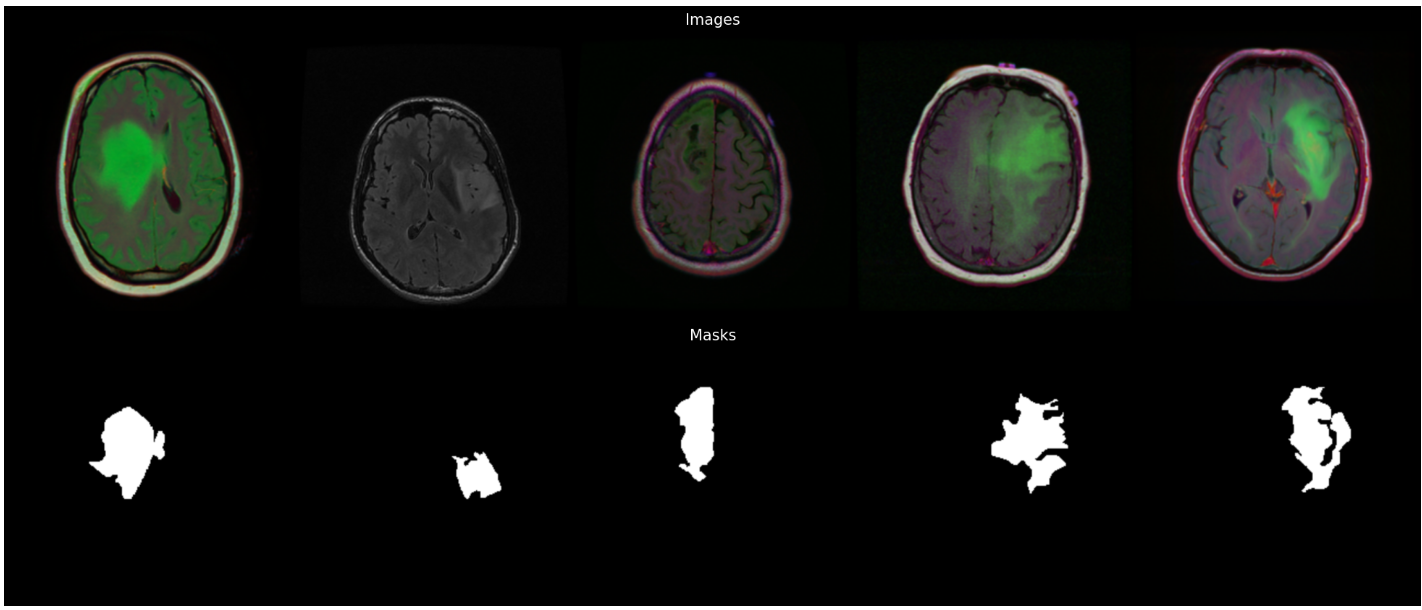
(9) 提取形状特征
sample_df = imagePath_df[imagePath_df["diagnosis"] == 1].sample(5).values
sample_imgs = []for i, data in enumerate(sample_df):#print(data)img = cv2.resize(cv2.imread(data[3]), (IMG_SIZE, IMG_SIZE))mask = cv2.resize(cv2.imread(data[4]), (IMG_SIZE, IMG_SIZE))sample_imgs.extend([img, mask])# Convert to grayscale if necessarygray_img = cv2.cvtColor(mask, cv2.COLOR_BGR2GRAY)# Threshold the image to obtain a binary mask_, binary_mask = cv2.threshold(gray_img, 128, 255, cv2.THRESH_BINARY)print(binary_mask.shape)result_MF = calculate_MF(binary_mask/ 255)result_ASD = calculate_ASD(binary_mask/ 255)result_BEVR = calculate_BEVR(binary_mask/ 255)print(result_MF)print(result_ASD)print(result_BEVR)sample_imgs_arr = np.hstack(np.array(sample_imgs[::2]))
sample_masks_arr = np.hstack(np.array(sample_imgs[1::2]))fig = plt.figure(figsize=(25., 25.))
grid = ImageGrid(fig, 111,  # similar to subplot(111)nrows_ncols=(2, 1),  # creates 2x2 grid of axesaxes_pad=0.1,  # pad between axes in inch.)grid[0].imshow(sample_imgs_arr)
grid[0].set_title("Images", fontsize=15)
grid[0].axis("off")
grid[1].imshow(sample_masks_arr)
grid[1].set_title("Masks", fontsize=15, y=0.9)
grid[1].axis("off")
plt.savefig(r"E:\工作\硕士\Brain-MRI-Segmentation-using-Deep-Learning-main\Masks.png",dpi=600,orientation='landscape')
输出结果:
更多优质内容持续发布中,请移步主页查看。
若有问题可邮箱联系:1736732074@qq.com
博主的WeChat:TCB1736732074
点赞+关注,下次不迷路!